

SITCOMTN-177
Covariance Estimation for AOS Closed-Loop OFC#
Abstract
This technote documents the estimation and validation of a noise covariance
matrix for use in the Optical Feedback Control (OFC) system of the Vera C.
Rubin Observatory Active Optics System (AOS). The covariance matrix
characterizes the uncertainty of wavefront measurements and is used by the
OFC StateEstimator to weight corrections during closed-loop operations.
Using on-sky stability test data from October–November 2025, we construct
both a full covariance matrix and an environment-clipped variant filtered
by seeing conditions. The matrices are validated against simulated
covariances and exported in YAML format for integration with ts_ofc
and ts_mtaos.
The companion notebook notebooks/covariance_estimation_analysis.ipynb
contains the detailed analysis and can be used to regenerate the results.
Introduction#
This technote is part of the AOS Closed-Loop Optimization effort. The parent task (RSO-99, Covariance Estimation) aims to use a measured noise covariance matrix inside the Optical Feedback Control (OFC) system to properly weight wavefront measurements during closed-loop operations.
The OFC system in ts_ofc uses a
StateEstimator to infer degrees of freedom (DOFs) – hexapod positions
and mirror bending modes – from wavefront Zernike coefficients measured by
the four corner wavefront sensors (R00, R04, R40, R44). By default, the
estimator assumes uniform measurement noise. Providing an explicit noise
covariance matrix allows the estimator to weight each Zernike mode and each
corner sensor according to its actual measurement uncertainty, improving the
accuracy and stability of closed-loop corrections.
This technote documents:
The construction of a noise covariance matrix from on-sky stability test data
Comparison of DOF state estimates using measured vs simulated covariance
The effect of environment-clipped covariances (filtered by seeing conditions)
The YAML export format for integration with
ts_ofc/ts_mtaos
The detailed computations are in the companion notebook
notebooks/covariance_estimation_analysis.ipynb.
Covariance Matrix Construction#
This chapter describes the data collection, processing, and covariance matrix construction pipeline.
Data Collection#
LSSTCam corner wavefront sensor Zernike coefficients (Z4–Z26, four corners: R00, R04, R40, R44) are fetched from the Butler and ConsDB across multiple stability test nights from October–November 2025.
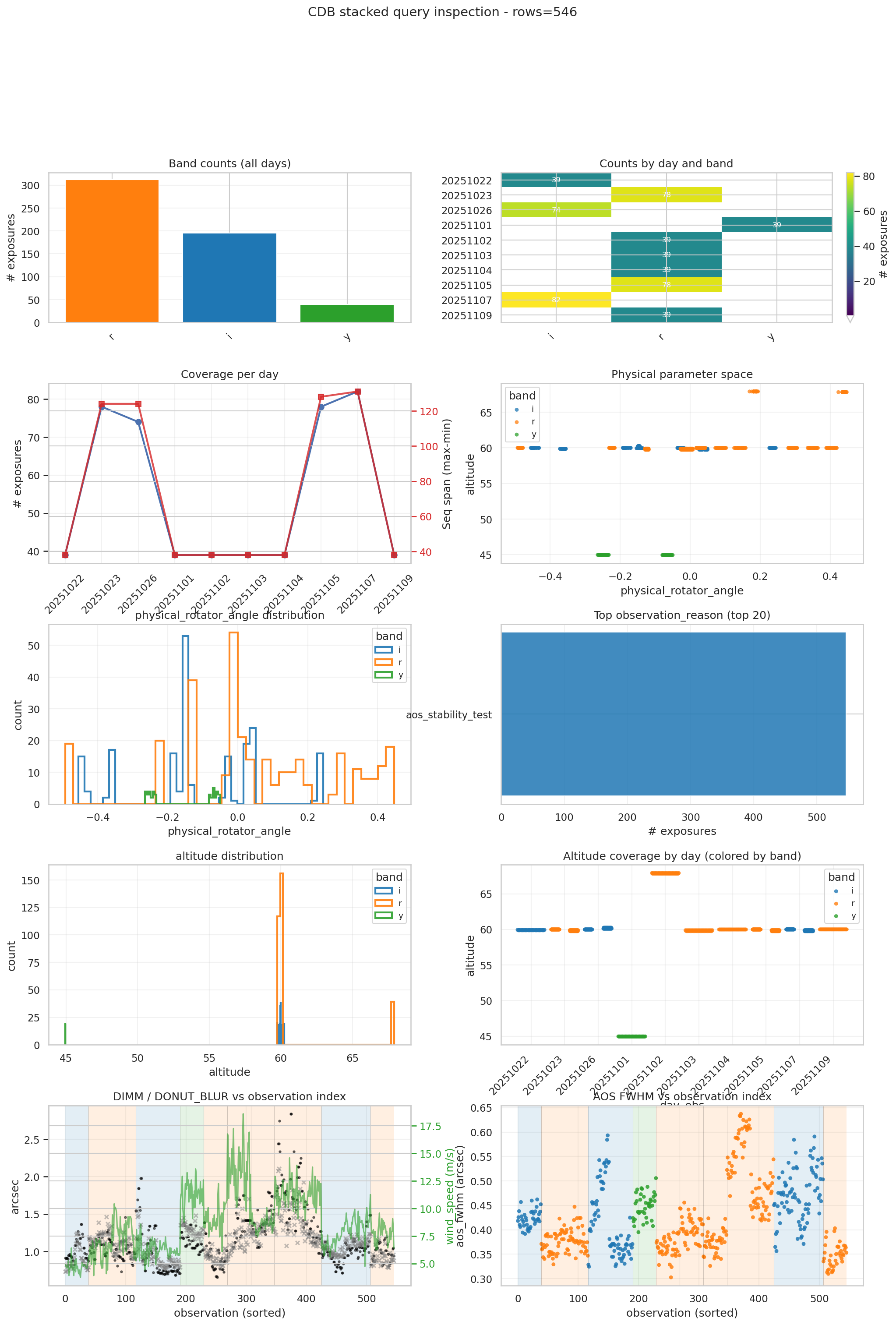
Fig. 1 Overview of the stability test nights used for covariance estimation, showing the available data blocks and sequence ranges.#
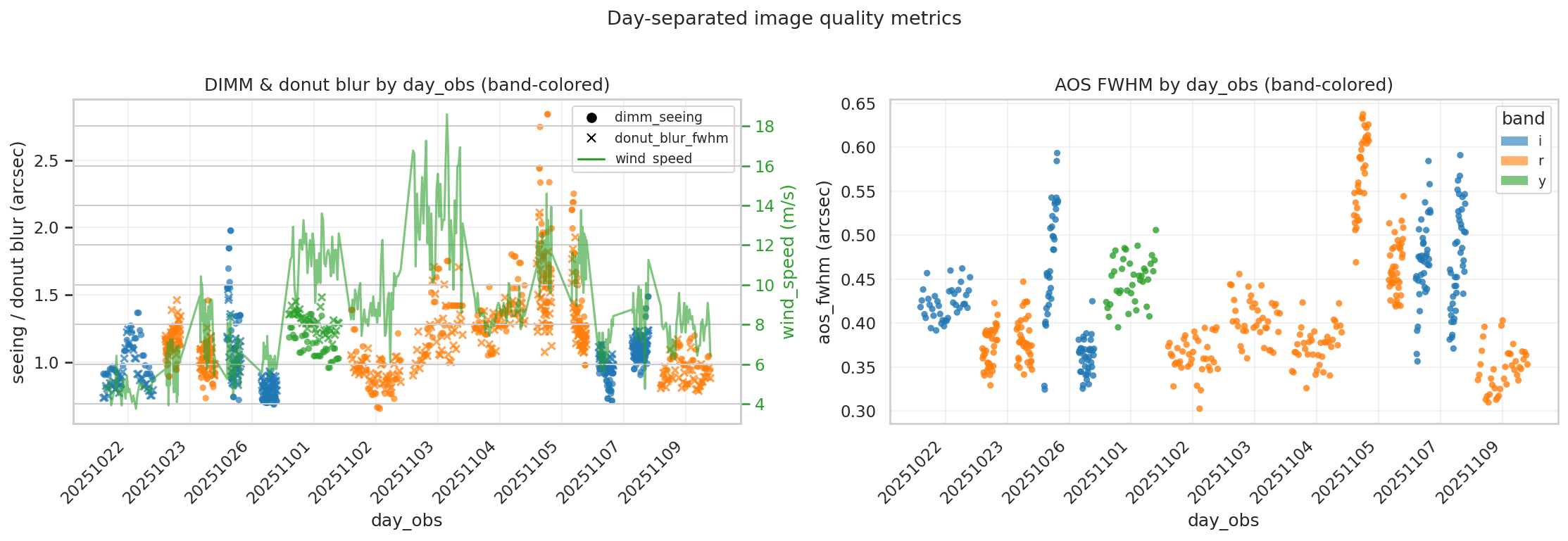
Fig. 2 Day-separated seeing and AOS metrics (donut blur FWHM, DIMM seeing), color-coded by band.#
Detrending#
Before computing the covariance, Zernike time series are detrended to remove slow drifts (e.g., thermal evolution, tracking errors) that would inflate variance estimates. A rolling median filter is applied to each coefficient independently.
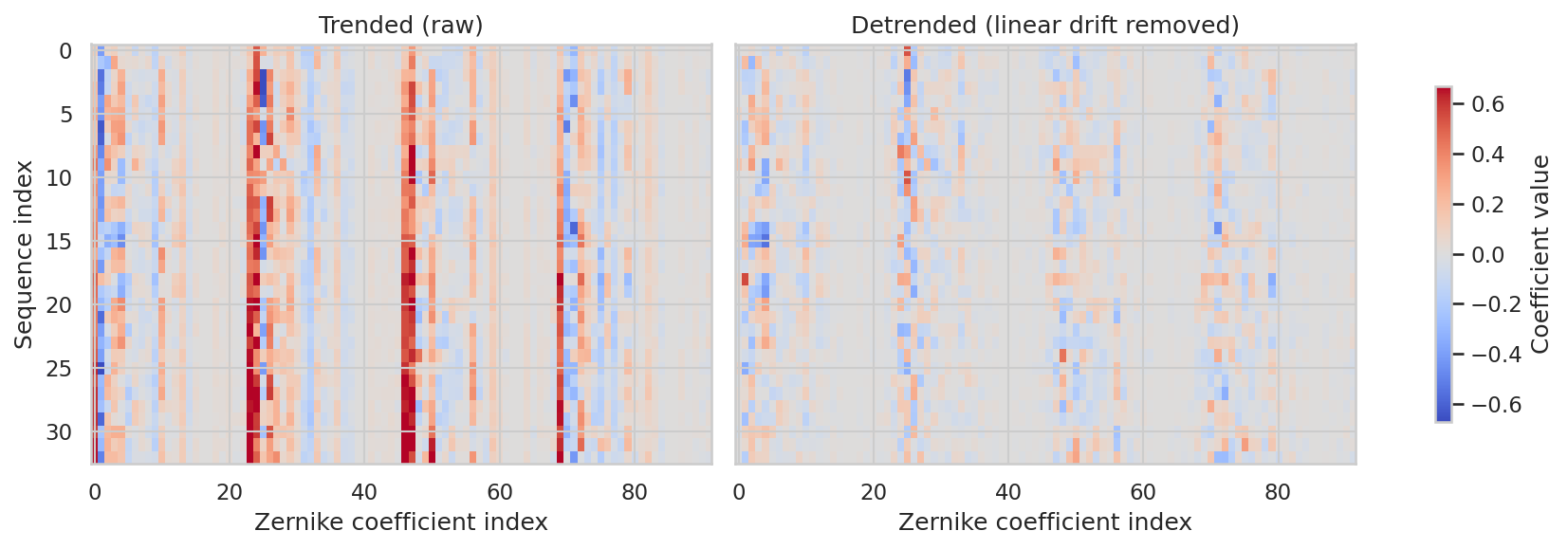
Fig. 3 Comparison of Zernike coefficients before (trended) and after (detrended) for a representative stability block.#
Covariance Matrix Construction#
The noise covariance matrix \(\mathbf{C}_n\) characterizes the measurement uncertainty of the wavefront Zernike coefficients. It tells the state estimator which Zernikes and corners are noisy (large diagonal entries) and which are correlated (large off-diagonal entries), enabling appropriate down-weighting during state estimation.
Given \(N\) exposures of detrended Zernike measurements, the sample covariance is estimated as:
where \(\mathbf{y}_k\) is the 92-element Zernike vector (23 Zernikes × 4 corners) for exposure \(k\), and \(\bar{\mathbf{y}}\) is the sample mean across all exposures.
The diagonal elements \([\hat{\mathbf{C}}_n]_{ii}\) represent the variance of each Zernike coefficient at each corner. The off-diagonal elements \([\hat{\mathbf{C}}_n]_{ij}\) capture correlations between different Zernikes or different corners — for example, common-mode atmospheric effects that affect all corners similarly, or optical aberrations that couple specific Zernike modes.
In the notebook, this is computed using np.cov(data, rowvar=False) on
the stacked detrended Zernike arrays from all stability nights, maximizing
the sample size for a robust estimate.
For a detailed mathematical description of how this covariance matrix is used in the OFC state estimator, see SOTN-001: OFC Control Loop Mathematical Description, Section 2.2.
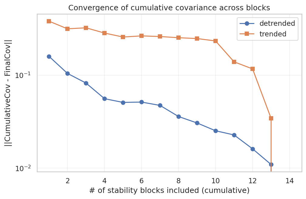
Fig. 4 Cumulative covariance matrix built from all stability blocks. The block structure reflects the four corner sensors, with each block showing Zernike-to-Zernike correlations within and across corners.#
Remapping to the OFC Target Grid#
The measured covariance (Z4–Z26, 23 modes) is remapped to the OFC target range (Z4–Z28, 25 modes). Missing modes (Z27, Z28) and zero-valued modes (Z20, Z21, which are not measured by the wavefront sensors) are assigned diagonal variance = 1 and off-diagonal covariance = 0. This ensures the matrix is invertible without affecting the state estimates for the truncated modes.
Corner-Order Canonicalization#
The covariance matrix is permuted from the historical data order
[R00, R40, R04, R44] to the ts_ofc canonical order [R00, R04, R40, R44].
This step is critical for compatibility with the StateEstimator.
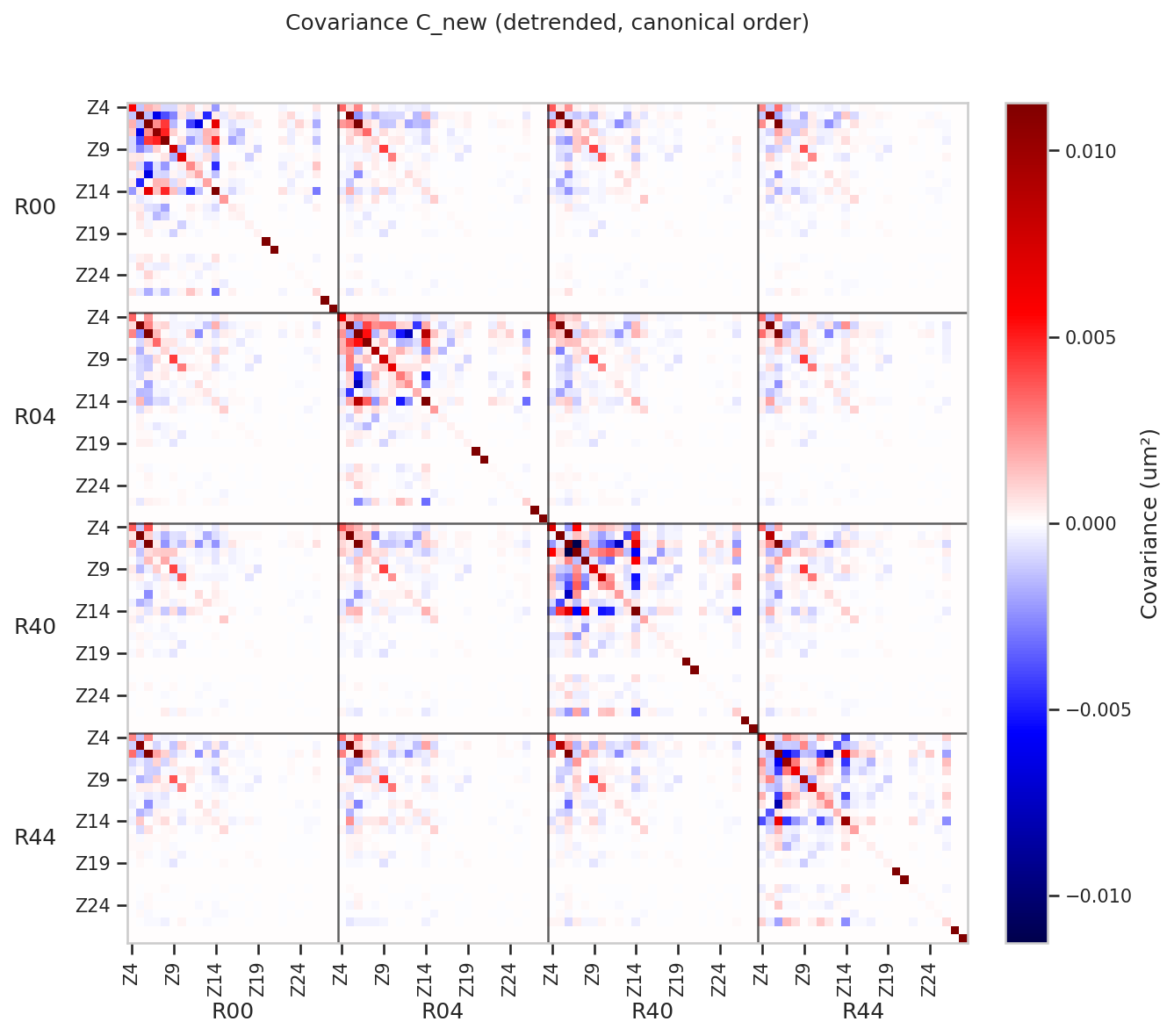
Fig. 5 The final covariance matrix C_new in canonical corner order.
The 4x4 block structure (one block per corner pair) is visible, with
each block containing 25x25 Zernike covariances.#
YAML Export Format#
The covariance matrix is exported to YAML for use by ts_ofc and
ts_mtaos. The format matches the existing
default_noise_covariance.yaml in ts_config_mttcs.
The YAML header documents:
Matrix dimensions and Zernike range
Corner ordering
Row index mapping (which rows correspond to which corner/Zernike)
Data provenance (nights, sequence ranges, clipping criteria)
Number of data points used
Example header:
---
 # Measurement noise covariance matrix (environment-clipped).
 # Clipping: donut_blur_fwhm <= 1.25 and 55 < altitude < 65
 # data_points = 142 (number of data points used to build this matrix)
 # Dimensions: (25*4,25*4) = (100,100). From j_min = 4 to j_max = 28.
 # Corner order: ['R00', 'R04', 'R40', 'R44'] (canonical ts_ofc)
 #
 # Each row is a YAML array '- [...]' representing one row of the
 # covariance matrix. The indexing is blocked by corner, with
 # 25 Zernikes (Z4-Z28) per corner:
 #
 #   Row indices  |  Meaning
 #   -------------|-------------------
 #   0-24          |  Z4-Z28 at corner R00
 #   25-49         |  Z4-Z28 at corner R04
 #   50-74         |  Z4-Z28 at corner R40
 #   75-99         |  Z4-Z28 at corner R44
 #
 # Night -> Sequence ranges (after clipping):
 # 20251022 : 206-244
 # 20251023 : 156-194, 242-280
 # ...
Each subsequent line is a YAML array - [v0, v1, ..., v99] representing
one row of the 100x100 covariance matrix.
State Estimation Comparison#
This chapter compares DOF state estimates under different noise covariance assumptions.
Overview#
The StateEstimator.dof_state() method in ts_ofc estimates the
optical system state (hexapod positions, mirror bending modes) from
wavefront Zernike measurements. The noise covariance matrix determines
how measurements are weighted in the least-squares estimation.
Three covariance configurations are compared:
Cov=False: No noise covariance (uniform weighting, equivalent to ordinary least squares)
SimCov: The pre-existing simulated covariance matrix from
ts_config_mttcsMeasuredCov: The newly measured covariance from on-sky stability data
Simulated vs Measured Covariance#
Before comparing state estimates, we examine the covariance matrices themselves.
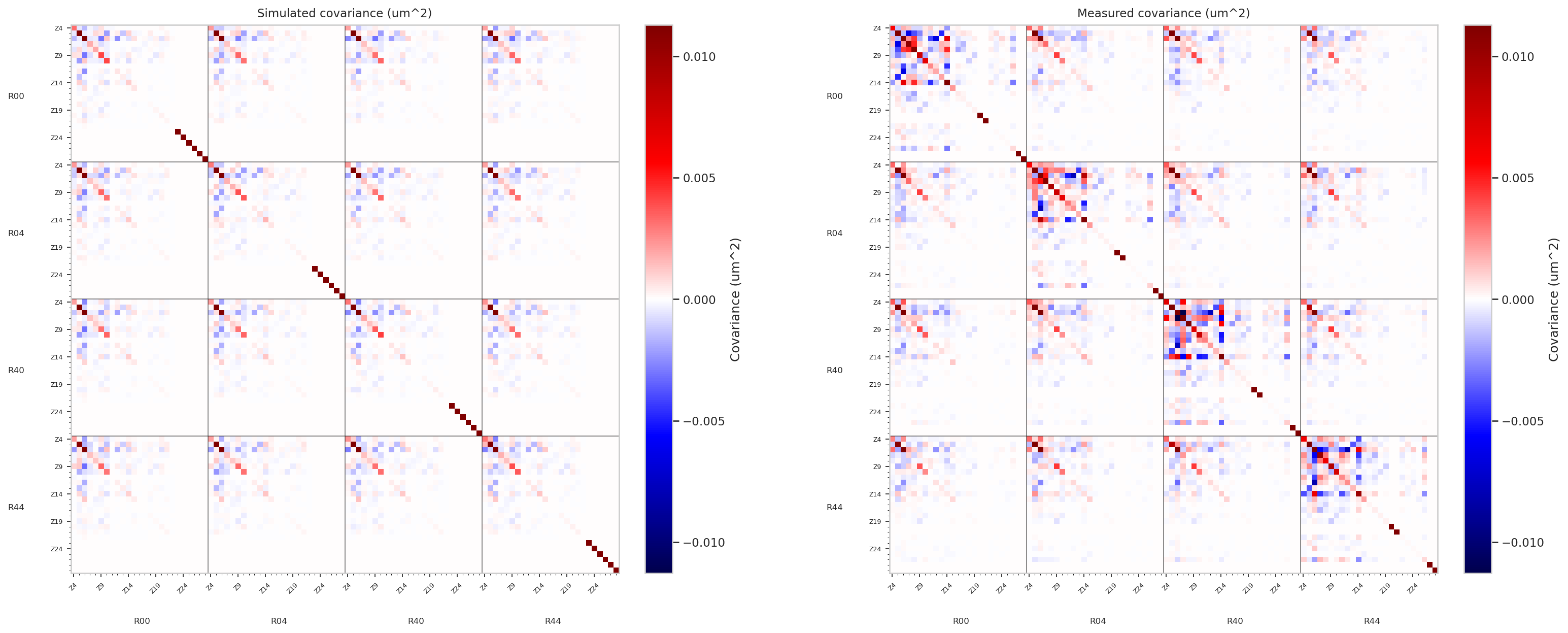
Fig. 6 Side-by-side comparison of simulated and measured covariance matrices. The simulated matrix is smoother (derived from optical models), while the measured matrix captures actual on-sky correlations including atmospheric and instrumental effects.#
DOF State Distributions#
State estimates are computed for all stability test exposures under each covariance configuration. The per-DOF distributions reveal how the covariance affects the estimated system state.
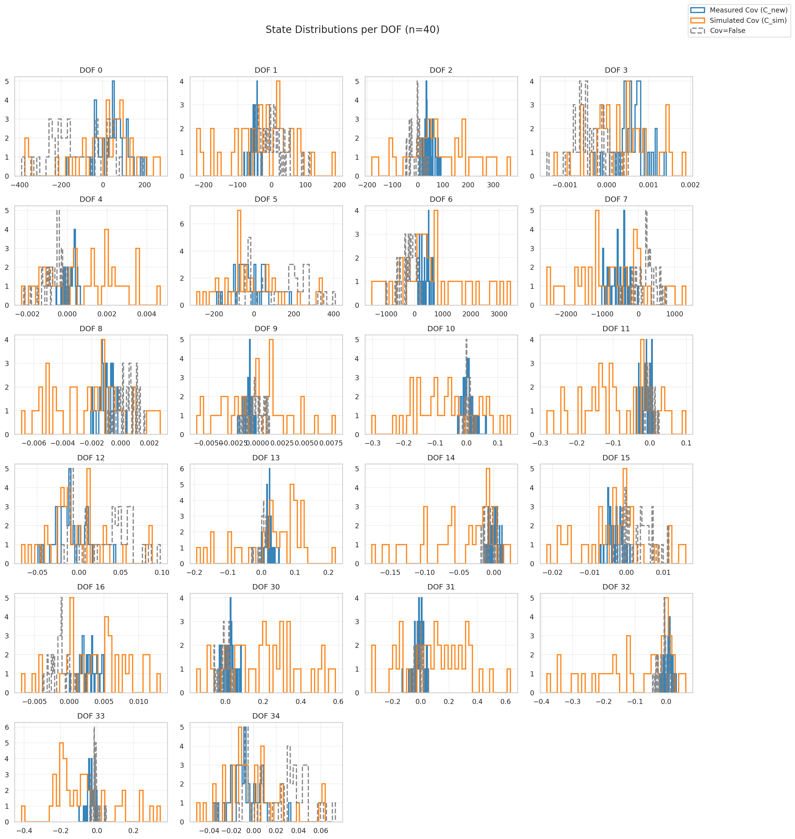
Fig. 7 Per-DOF state distributions comparing Cov=False (baseline), SimCov, and MeasuredCov. The distributions show:#
Width changes: Different effective weighting of Zernike modes
Mean shifts: Potential biases in the estimation
Tail behavior: Sensitivity to outliers
Key Findings#
The measured covariance produces DOF estimates that are generally consistent with the simulated covariance, validating the simulation assumptions.
Some DOFs show modest differences between SimCov and MeasuredCov, reflecting real on-sky correlations not captured by the simulation.
Using any covariance (SimCov or MeasuredCov) produces more stable estimates than Cov=False for higher-order modes, where the uniform weighting amplifies noise.
Environment-Clipped Covariance Analysis#
This chapter investigates how covariance matrices built from subsets of data (clipped by observing conditions) affect DOF state estimates.
Motivation#
The measurement noise covariance depends on observing conditions. During poor seeing, wavefront measurements have higher variance and different correlation structure than during good seeing. Building a covariance matrix from a specific subset of conditions may better represent the expected noise during similar future observations.
Clipping Criteria#
Environment-clipped covariance matrices are built using two filters:
Donut blur FWHM: Bins at <= 1.0, 1.0–1.25, 1.25–1.5, and > 1.5 arcsec
Altitude window: Optional elevation range (e.g., 55–65 degrees)
An “aggregate” clipped covariance is also computed using all data with donut blur <= 1.25 arcsec (good-to-moderate seeing).
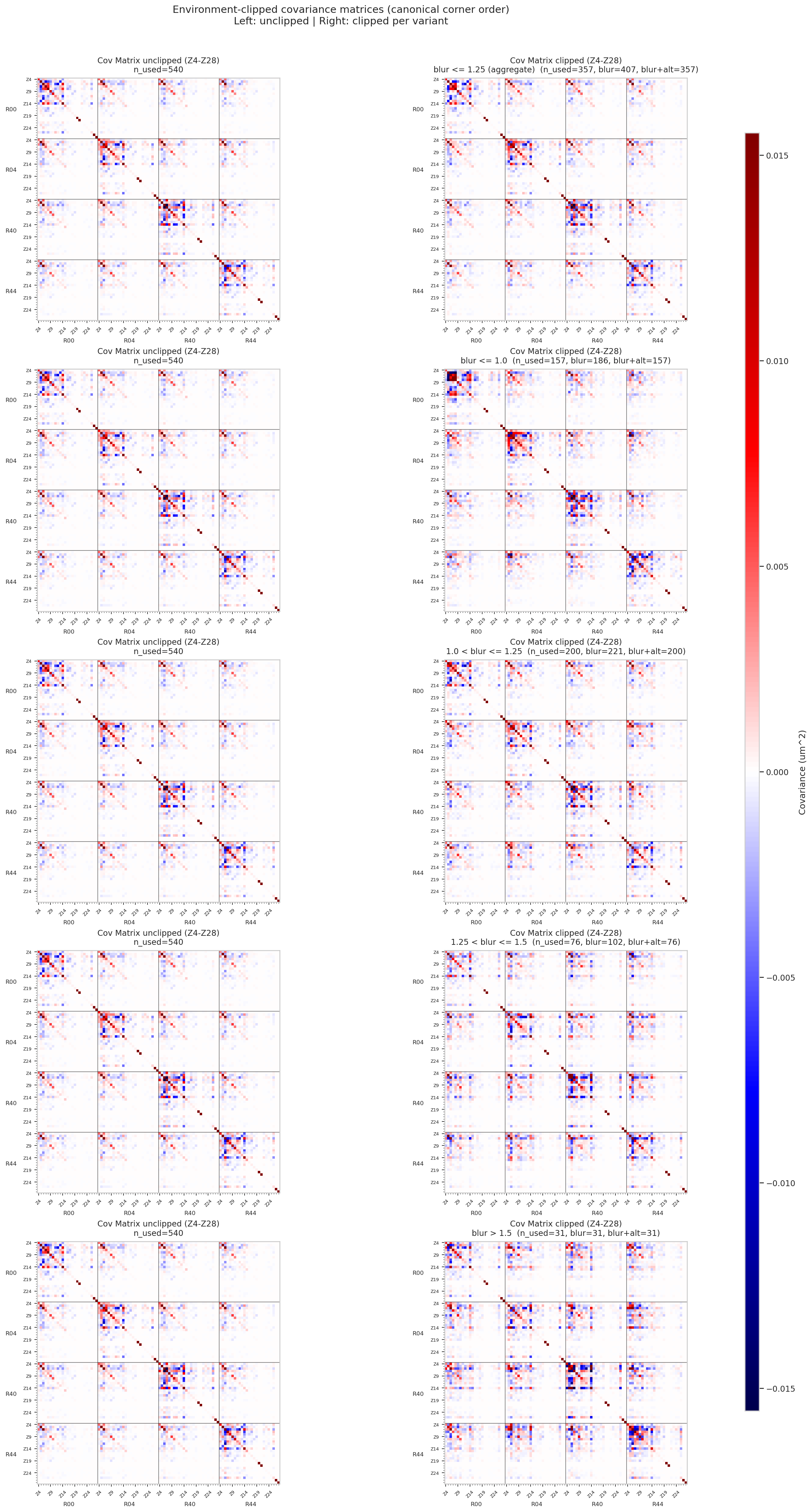
Fig. 8 Side-by-side comparison of covariance matrices for each blur bin. Left column: unclipped reference. Right column: clipped variant. The covariance structure changes with seeing conditions – better seeing (lower blur) produces lower overall variance and tighter correlations.#
DOF State Comparison#
State estimates are recomputed using each clipped covariance variant and compared to the baseline (Cov=False) and unclipped covariance.
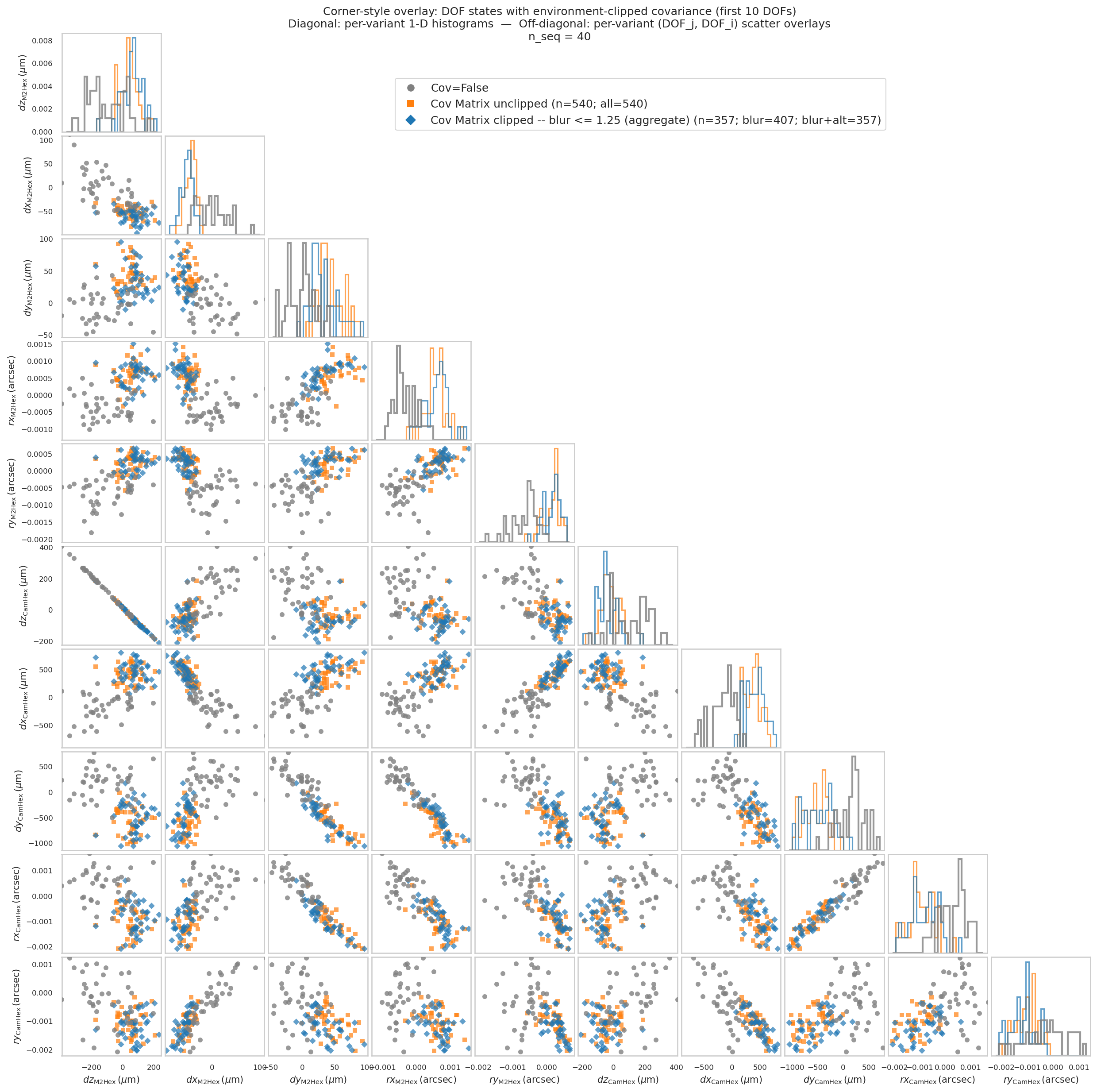
Fig. 9 Corner-style overlay plot comparing DOF state distributions across covariance variants:#
Cov=False (baseline)
Unclipped (all data)
Aggregate clipped (blur <= 1.25 arcsec)
Positive Semi-Definiteness Constraint#
A valid noise covariance matrix must be positive semi-definite (PSD) – all eigenvalues must be non-negative. When the number of data points used to build the covariance is too small relative to the matrix dimension (100x100 = 10,000 elements), the resulting matrix may fail to be PSD due to sampling noise.
This occurs in practice for the stricter blur bins (e.g., blur <= 1.0 arcsec) combined with altitude windowing, where only a few dozen data points may survive the filters. The notebook reports PSD status for each clipped variant and skips non-PSD matrices in state estimation comparisons.
Note
For production use, the recommended covariance is the aggregate clipped variant (blur <= 1.25 arcsec with altitude windowing), which balances data quality filtering with sufficient sample size for a stable PSD matrix.
Conclusions#
Environment clipping is effective: Covariance matrices built from good-seeing subsets have lower diagonal variance and cleaner off-diagonal structure.
Sample size matters: Aggressive clipping (blur <= 1.0 arcsec) can produce non-PSD matrices when combined with altitude windowing. The aggregate clipped variant (blur <= 1.25 arcsec) provides a good balance.
DOF estimates are robust: The estimated DOF states are relatively insensitive to the choice of clipped vs unclipped covariance, suggesting the measurement correlations are well-characterized across conditions.
Recommendation: Use the aggregate clipped covariance (
onsky_stability_covariance_clipped.yaml) for closed-loop operations. It represents typical good-seeing conditions and has been validated as PSD.
Conclusions and Deliverables#
Summary#
This technote documents the estimation and validation of a noise covariance
matrix for the OFC StateEstimator from on-sky stability test data.
Key findings:
Measured covariance is consistent with simulation: The on-sky measured covariance matrix shows similar structure to the pre-existing simulated covariance, validating the simulation assumptions.
Environment clipping improves covariance quality: Filtering data by donut blur FWHM (good-seeing conditions) produces cleaner covariance estimates with lower variance.
Sample size constraints: Aggressive environment clipping can produce non-positive-definite matrices when the number of data points is insufficient. The recommended aggregate clipped variant (blur <= 1.25 arcsec, altitude 55–65 degrees) balances quality filtering with statistical stability.
DOF estimates are robust: State estimation results are relatively insensitive to the choice between simulated, measured, or clipped covariance variants, indicating the system is well-characterized.
Deliverables#
Two covariance matrices are provided in YAML format for integration with
ts_ofc and ts_mtaos:
onsky_stability_covariance.yaml: Full covariance built from all stability test data (no environment clipping).
onsky_stability_covariance_clipped.yaml: Aggregate clipped covariance built from good-seeing data (donut blur <= 1.25 arcsec, altitude 55–65 degrees). This is the recommended matrix for production use.
Both files are located in the notebook output directory
(covariance_state_estimation/) and follow the format expected by
ts_config_mttcs/MTAOS/ofc/noise_covariance/.
Future Work#
Operational validation: Deploy the measured covariance in closed-loop operations and compare on-sky performance to the simulated covariance.
Condition-dependent covariance: Investigate using different covariance matrices based on real-time seeing conditions.
Extended Zernike range: When higher-order Zernike measurements (Z27+) become available, update the covariance estimation to include them.
Appendix: Diagnostic Plots#
This appendix contains detailed diagnostic plots that support the main analysis but are not essential for understanding the core results.
Cross-Corner Correlation Analysis#
Pearson correlations between Zernike measurements at different corner sensors reveal common-mode vs local behavior.
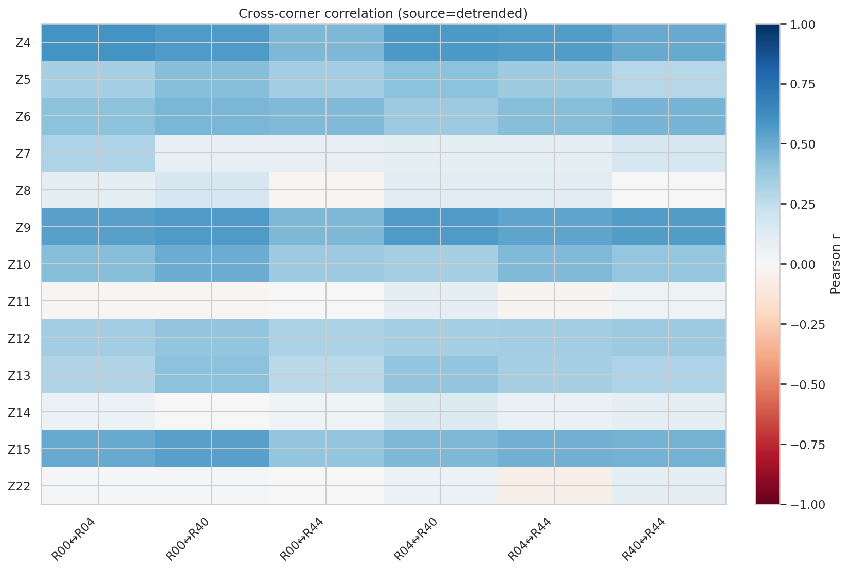
Fig. 10 Cross-corner correlation coefficients for each Zernike mode. High correlations indicate common-mode atmospheric or optical effects; low correlations indicate local sensor or field-dependent behavior.#
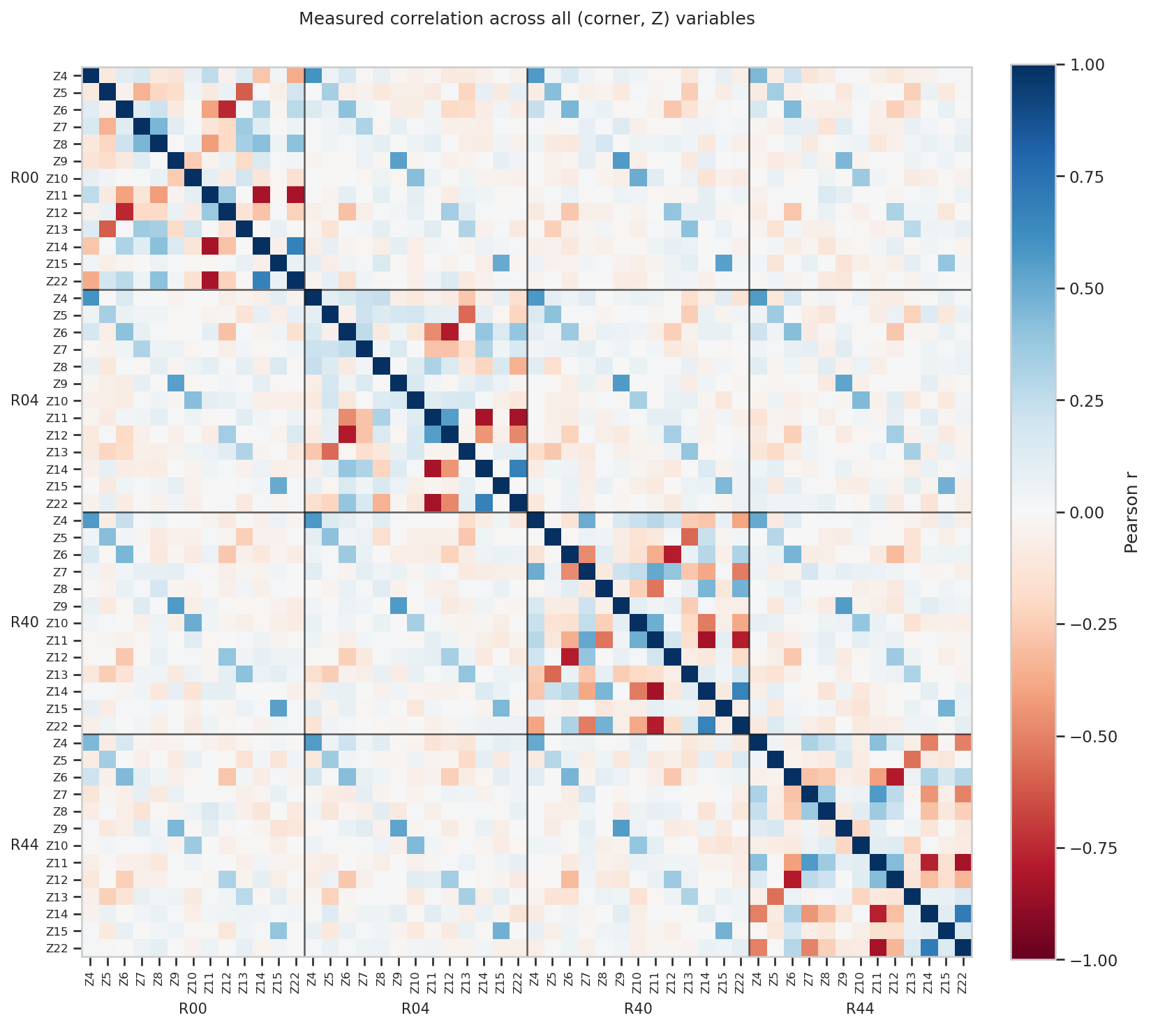
Fig. 11 Full correlation matrix across all (corner, Zernike) combinations. The block structure reflects corner groupings.#
Variance Comparison: Simulated vs Measured#
Per-corner, per-Zernike diagonal variance comparison between the simulated covariance (in nm^2) and measured covariance (in um^2, converted to nm^2).
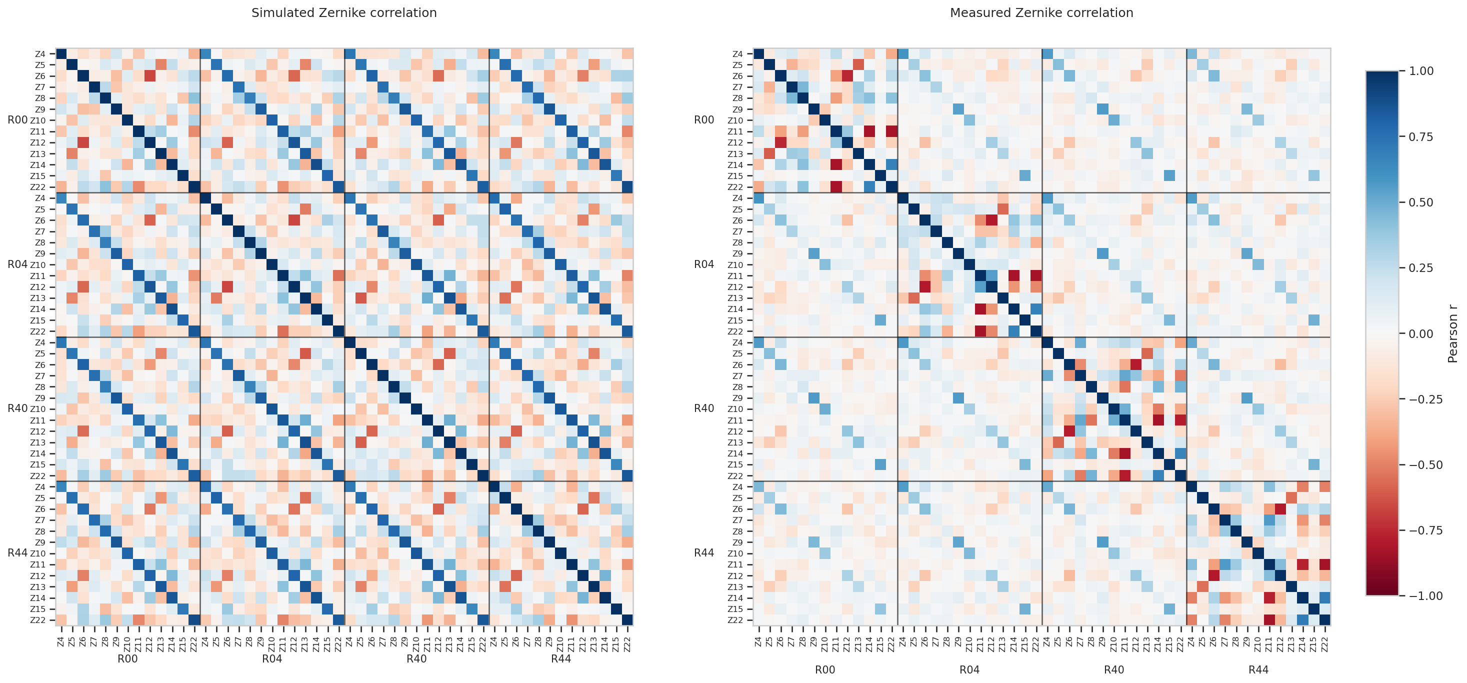
Fig. 12 Diagonal variance comparison. The simulated covariance was computed at 770nm wavelength; measured values are in um (OPD length units).#
Correlation Structure by Blur Bin#
The measured correlation matrix recomputed for different donut blur bins, showing how correlation structure changes with seeing conditions.
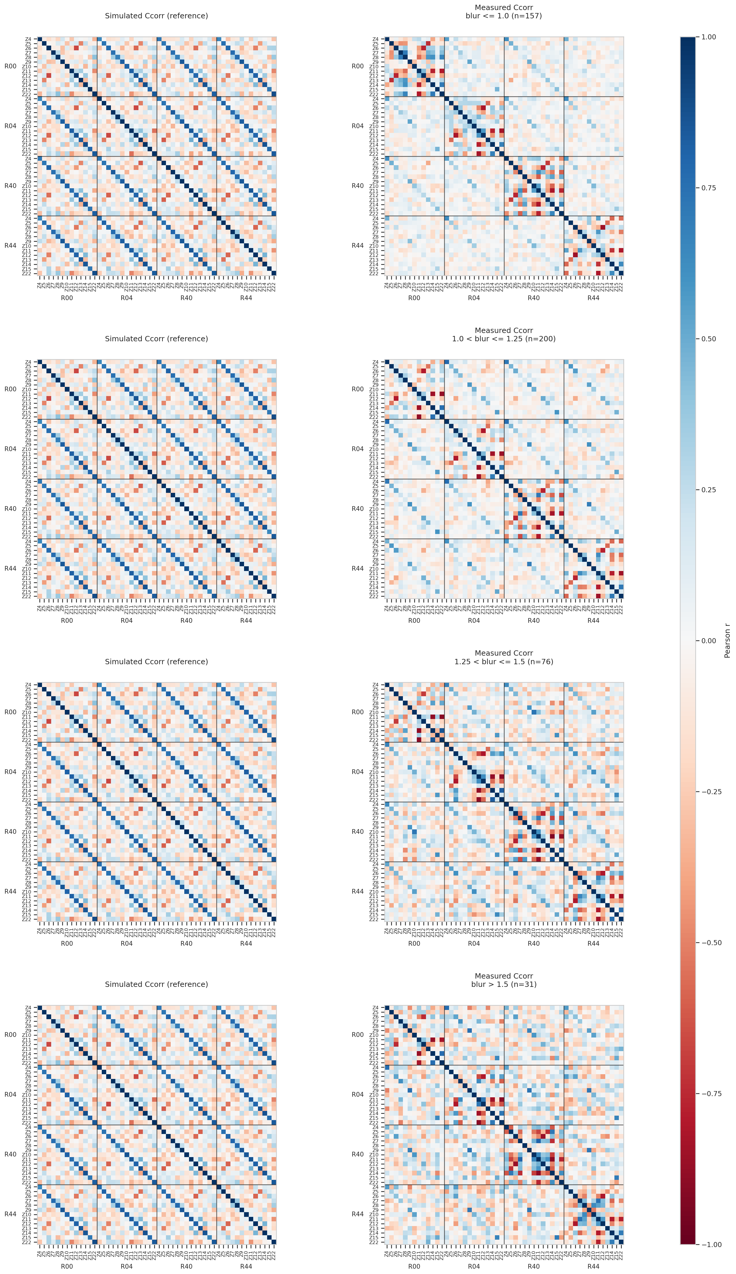
Fig. 13 Correlation matrices for different blur bins compared to the simulated reference. Worse seeing (higher blur) shows increased decorrelation.#
Per-Blur-Bin DOF Distributions#
Complete set of DOF distributions for all blur-bin clipped covariance variants (including those that may be non-PSD).
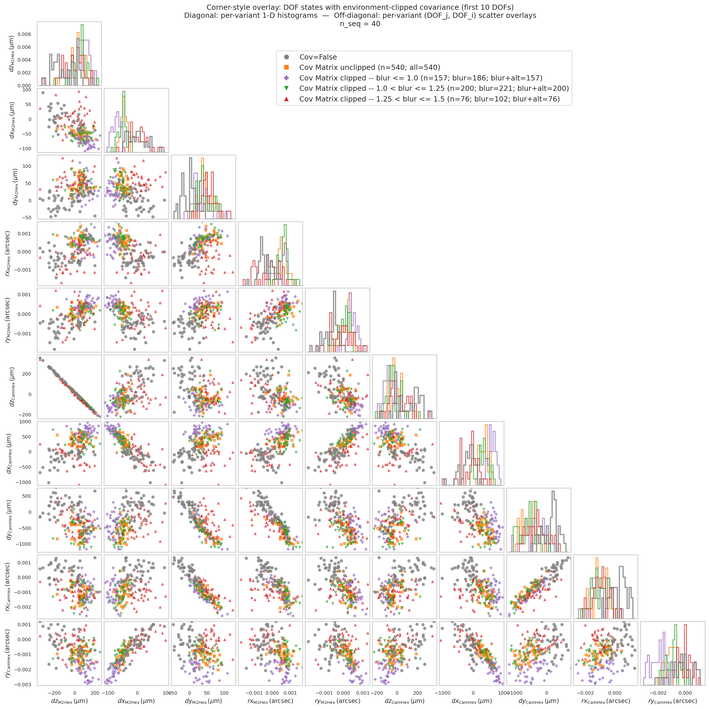
Fig. 14 Corner-style overlay including all per-blur-bin variants. Some variants may be excluded if their covariance matrix is not positive semi-definite.#